13. Example Application

13.1. Introduction

In this section, we compare the performance of two different control sequences. The objectives are to demonstrate the setup for closed loop performance assessment, to demonstrate how to compare control performance, and to assess the difference in annual energy consumption.

As a test case, we used a simulation model that consists of five thermal zones that are representative of one floor of the new construction medium office building for Chicago, IL, as described in the set of DOE Commercial Building Benchmarks [DFS+11]. There are four perimeter zones and one core zone. The envelope thermal properties meet ASHRAE Standard 90.1-2004. The system model consist of an HVAC system, a building envelope model [WZN11] and a model for air flow through building leakage and through open doors based on wind pressure and flow imbalance of the HVAC system [Wet06]. Thus, at every simulation step, a full pressure drop calculation is done to compute the air flow distribution based on damper positions, fan control signal and fan curve.

For the base case, we implemented a control sequence published in ASHRAE’s Sequences of Operation for Common HVAC Systems [ASH06]. For the other case, we implemented the control sequence published in ASHRAE Guideline 36 [ASHRAE16]. The main conceptual differences between the two control sequences, which are described in more detail in Section 13.2.5, are as follows:

• The base case uses two different but constant supply air temperature setpoints for heating and cooling during occupied hours, whereas Guideline 36 case resets the supply air temperature setpoint based on outdoor air temperature and zone cooling requests, as obtained from the VAV terminal unit controllers. The reset is using the trim and respond logic.

• The base case resets the supply fan static pressure setpoint based on the VAV damper positions, whereas the Guideline 36 case resets the fan static pressure setpoint based on zone pressure requests from the VAV terminal controllers. The reset is using the trim and respond logic.

• The base case controls the economizer to track a mixed air temperature setpoint, whereas Guideline 36 controls the economizer based on supply air temperature control loop signal.

• The base case controls the VAV dampers based on the zone’s cooling temperature setpoint, whereas Guideline 36 uses the heating and cooling loop signal to control the VAV dampers.

The next sections are as follows: In Section 13.2 we describe the methodology, the models and the performance metrics, in Section 13.3 we compare the performance, in Section 13.4 we recommend improvements to the Guideline 36 and in Section 13.5 we discuss the main findings and present concluding remarks.

13.2. Methodology

All models are implemented in Modelica, using models from the Buildings library [WZNP14]. The models are available from https://github.com/lbl-srg/modelica-buildings/releases/tag/v5.0.0

13.2.1. HVAC Model

The HVAC system is a variable air volume (VAV) flow system with economizer and a heating and cooling coil in the air handler unit. There is also a reheat coil and an air damper in each of the five zone inlet branches.

Fig. 13.1 shows the schematic diagram of the HVAC system.

Fig. 13.1 Schematic diagram of the HVAC system.

In the VAV model, all air flows are computed based on the duct static pressure distribution and the performance curves of the fans. The fans are modeled as described in [Wet13].

13.2.2. Envelope Heat Transfer

The thermal room model computes transient heat conduction through walls, floors and ceilings and long-wave radiative heat exchange between surfaces. The convective heat transfer coefficient is computed based on the temperature difference between the surface and the room air. There is also a layer-by-layer short-wave radiation, long-wave radiation, convection and conduction heat transfer model for the windows. The model is similar to the Window 5 model. The physics implemented in the building model is further described in [WZN11].

There is no moisture buffering in the envelope, but the room volume has a dynamic equation for the moisture content.

13.2.3. Internal Loads

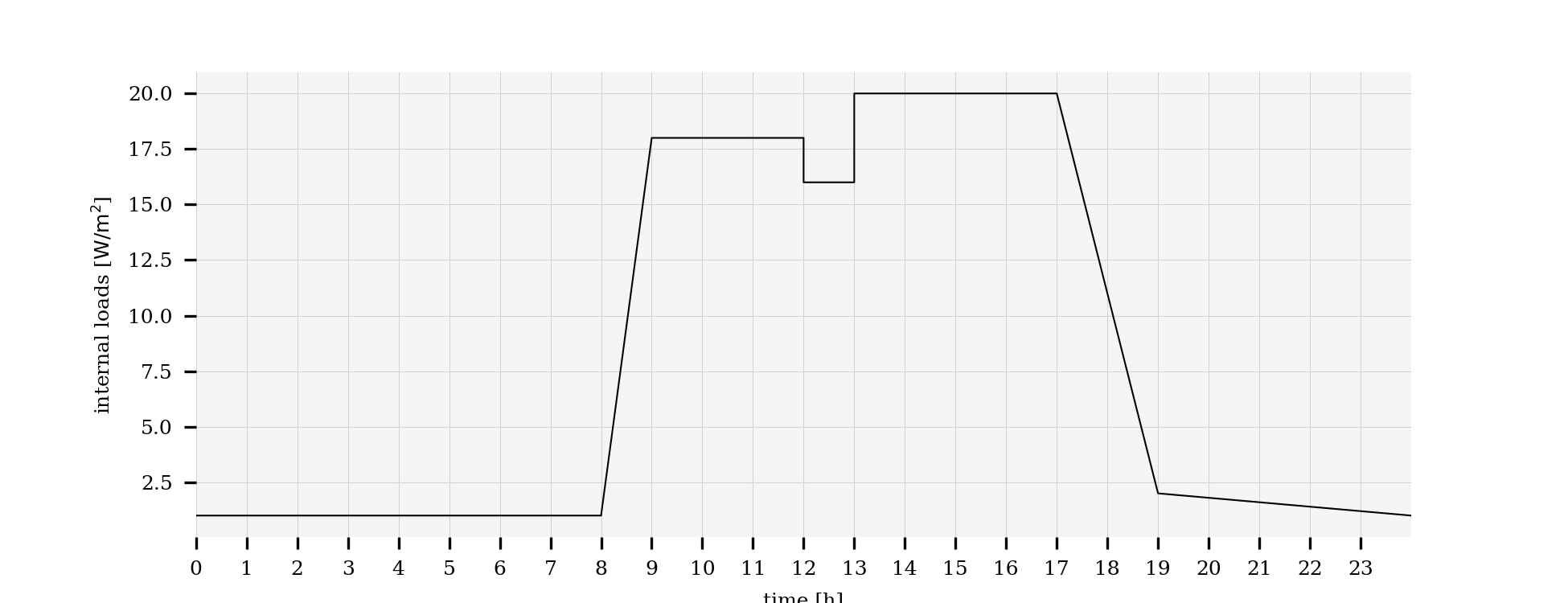
Fig. 13.2 Internal load schedule.

We use an internal load schedule as shown in Fig. 13.2, of which \(20\%\) is radiant, \(40\%\) is convective sensible and \(40\%\) is latent. Each zone has the same internal load per floor area.

13.2.4. Multi-Zone Air Exchange

Each thermal zone has air flow from the HVAC system, through leakages of the building envelope (except for the core zone) and through bi-directional air exchange through open doors that connect adjacent zones. The bi-directional air exchange is modeled based on the differences in static pressure between adjacent rooms at a reference height plus the difference in static pressure across the door height as a function of the difference in air density. Air infiltration is a function of the flow imbalance of the HVAC system. The multizone airflow models are further described in [Wet06].

13.2.5. Control Sequences

For the above models, we implemented two different control sequences, which are described below. The control sequences are the only difference between the two cases.

For the base case, we implemented the control sequence VAV 2A2-21232 of the Sequences of Operation for Common HVAC Systems [ASH06]. In this control sequence, the supply fan speed is modulated to maintain a duct static pressure setpoint. The duct static pressure setpoint is adjusted so that at least one VAV damper is 90% open. The economizer dampers are modulated to track the setpoint for the mixed air dry bulb temperature. The supply air temperature setpoints for heating and cooling are constant during occupied hours, which may not comply with some energy codes. Priority is given to maintain a minimum outside air volume flow rate. In each zone, the VAV damper is adjusted to meet the room temperature setpoint for cooling, or fully opened during heating. The room temperature setpoint for heating is controlled by varying the water flow rate through the reheat coil. There is also a finite state machine that transitions the mode of operation of the HVAC system between the modes occupied, unoccupied off, unoccupied night set back, unoccupied warm-up and unoccupied pre-cool. Local loop control is implemented using proportional and proportional-integral controllers, while the supervisory control is implemented using a finite state machine.

For the detailed implementation of the control logic, see the model Buildings.Examples.VAVReheat.ASHRAE2006, which is also shown in Fig. 13.6.

Our implementation differs from VAV 2A2-21232 in the following points:

• We removed the return air fan as the building static pressure is sufficiently large. With the return fan, building static pressure was not adequate.

• In order to have the identical mechanical system as for the Guideline 36 case, we do not have a minimum outdoor air damper, but rather controlled the outdoor air damper to allow sufficient outdoor air if the mixed air temperature control loop would yield too little outdoor air.

For the Guideline 36 case, we implemented the multi-zone VAV control sequence based on [ASHRAE16]. Fig. 13.3 shows the sequence diagram, and the detailed implementation is available in the model Buildings.Examples.VAVReheat.Guideline36.

In the Guideline 36 sequence, the duct static pressure is reset using trim and respond logic based on zone pressure reset requests, which are issued from the terminal box controller based on whether the measured flow rate tracks the set point. The implementation of the controller that issues these system requests is shown in Fig. 13.4. The economizer dampers are modulated based on a control signal for the supply air temperature set point, which is also used to control the heating and cooling coil valve in the air handler unit. Priority is given to maintain a minimum outside air volume flow rate. The supply air temperature setpoints for heating and cooling at the air handler unit are reset based on outdoor air temperature, zone temperature reset requests from the terminal boxes and operation mode.

In each zone, the VAV damper and the reheat coil is controlled using the sequence shown in Fig. 13.5, where THeaSet is the set point temperature for heating, dTDisMax is the maximum temperature difference for the discharge temperature above THeaSet, TSup is the supply air temperature, VAct* are the active airflow rates for heating (Hea) and cooling (Coo), with their minimum and maximum values denoted by Min and Max.

Fig. 13.3 Control schematics of Guideline 36 case.

Fig. 13.4 Composite block that implements the sequence for the VAV terminal units that output the system requests. (Browsable version.)

Fig. 13.5 Control sequence for VAV terminal unit.

Our implementation differs from Guideline 36 in the following points:

• Guideline 36 prescribes “To avoid abrupt changes in equipment operation, the output of every control loop shall be capable of being limited by a user adjustable maximum rate of change, with a default of 25% per minute.”

  We did not implement this limitation of the output as it leads to delays which can make control loop tuning more difficult if the output limitation is slower than the dynamics of the controlled process. We did however add a first order hold at the trim and response logic that outputs the duct static pressure setpoint for the fan speed.

• Not all alarms are included.

• Where Guideline 36 prescribes that equipment is enabled if a controlled quantity is above or below a setpoint, we added a hysteresis. In real systems, this avoids short-cycling due to measurement noise, in simulation, this is needed to guard against numerical noise that may be introduced by a solver.

13.2.6. Site Electricity Use

To convert cooling and heating energy as transferred by the coil to site electricity use, we apply the conversion factors from EnergyStar [Ene13]. Therefore, for an electric chiller, we assume an average coefficient of performance (COP) of \(3.2\) and for a geothermal heat pump, we assume a COP of \(4.0\).

13.2.7. Simulations

Fig. 13.6 shows the top-level of the system model of the base case, and Fig. 13.7 shows the same view for the Guideline 36 model.

Fig. 13.6 Top level view of Modelica model for the base case.

Fig. 13.7 Top level view of Modelica model for the Guideline 36 case.

The complexity of the control implementation is visible in Fig. 13.4 which computes the temperature and pressure requests of each terminal box that is sent to the air handler unit control.

All simulations were done with Dymola 2018 FD01 beta3 using Ubuntu 16.04 64 bit. We used the Radau solver with a tolerance of \(10^{-6}\). This solver adaptively changes the time step to control the integration error. Also, the time step is adapted to properly simulate time events and state events.

The base case and the Guideline 36 case use the same HVAC and building model, which is implemented in the base class Buildings.Examples.VAVReheat.BaseClasses.PartialOpenLoop. The two cases differ in their implementation of the control sequence only, which is implemented in the models Buildings.Examples.VAVReheat.BaseClasses.ASHRAE2006 and Buildings.Examples.VAVReheat.BaseClasses.Guideline36.

Table 13.1 shows an overview of the model and simulation statistics. The differences in the number of variables and in the number of time varying variables reflect that the Guideline 36 control is significantly more detailed than what may otherwise be used for simulation of what the authors believe represents a realistic implementation of a feedback control sequence. The entry approximate number of control I/O connections counts the number of input and output connections among the control blocks of the two implementations. For example, If a P controller receives one set point, one measured quantity and sends it signal to a limiter and the limiter output is connected to a valve, then this would count as four connections. Any connections inside the PI controller would not be counted, as the PI controller is an elementary building block (see Section 7.6) of CDL.

Table 13.1 Model and simulation statistics.

Quantity	Base case	Guideline 36
Number of components	2826	4400
Number of variables (prior to translation)	33,700	40,400
Number of continuous states	178	190
Number of time-varying variables	3400	4800
Time for annual simulation in minutes	70	100

13.3. Performance Comparison

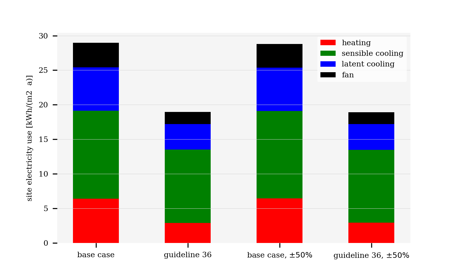
Fig. 13.8 Comparison of energy use. For the cases labeled \(\pm 50\%\), the internal gains have been increased and decreased as described in Section 13.2.3.

Table 13.2 Heating, cooling, fan and total site HVAC energy, and savings of guideline 36 case versus base case.

\(E_{h} \quad [kWh/(m^2\,a)]\)	\(E_{c} \quad [kWh/(m^2\,a)]\)	\(E_{f} \quad [kWh/(m^2\,a)]\)	\(E_{tot} \quad [kWh/(m^2\,a)]\)	[%]
6.419	18.98	3.572	28.97
2.912	14.29	1.74	18.94	34.6

Fig. 13.8 and Table 13.2 compare the annual site HVAC electricity use between the annual simulations with the base case control and the Guideline 36 control. The bars labeled \(\pm 50\%\) were obtained with simulations in which we changed the diversity of the internal loads. Specifically, we reduced the internal loads for the north zone by \(50\%\) and increased them for the south zone by the same amount.

In this case study, the Guideline 36 control saves around \(30\%\) site HVAC electrical energy. These are significant savings that can be achieved through software only, without the need for additional hardware or equipment. Our experience, however, was that it is rather challenging to program the Guideline 36 sequence due to their complex logic that contains various mode changes, interlocks and timers. Various programming errors and misinterpretations or ambiguities of Guideline 36 were only discovered in closed loop simulations. We therefore believe it is important to provide robust, validated implementations of Guideline 36 that encapsulates the complexity for the energy modeler and the control provider.

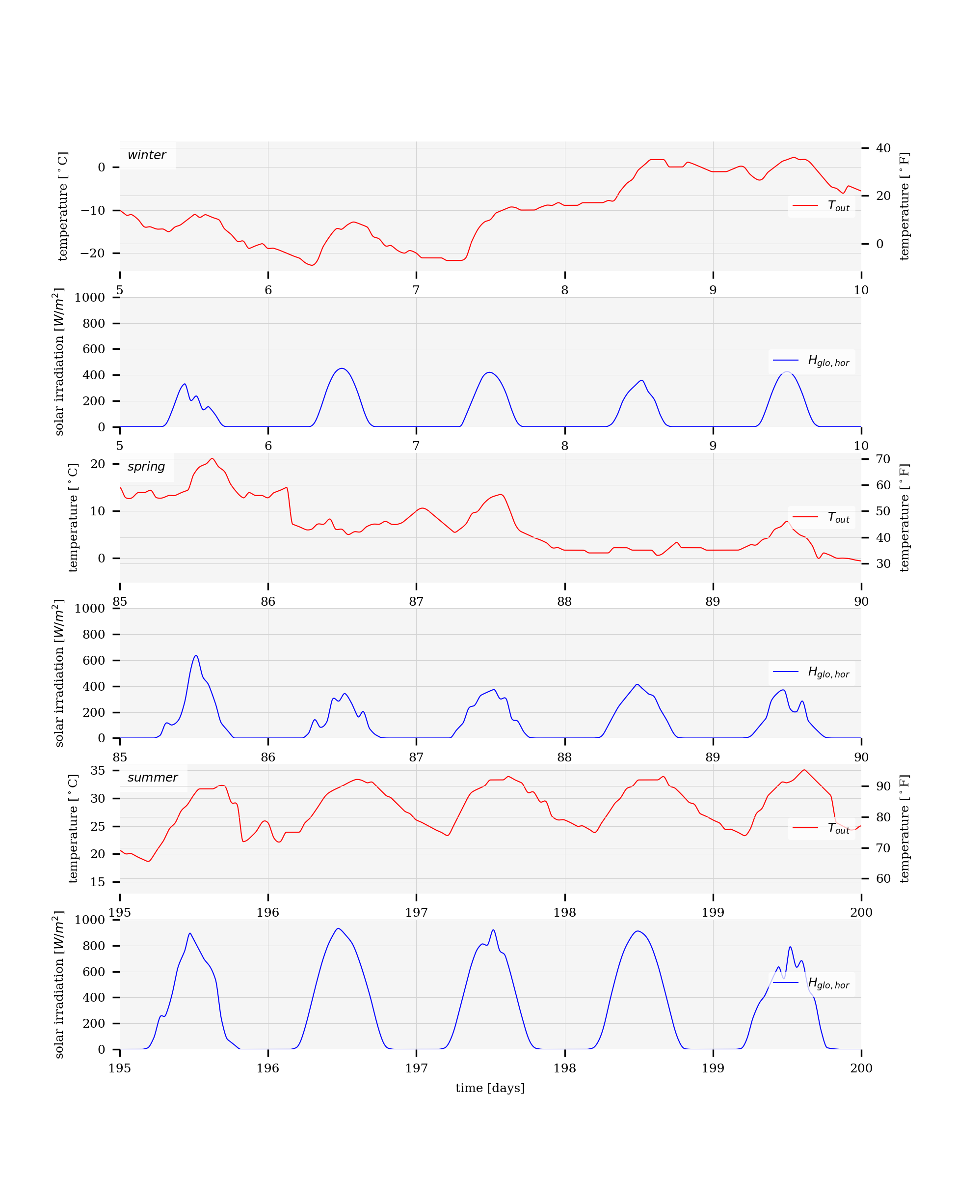
Fig. 13.9 Outside air temperature and global horizontal irradiation for the three periods that will be further used in the analysis.

Fig. 13.9 shows the outside air temperature temperature \(T_{out}\) and the global horizontal irradiation \(H_{glo,hor}\) for a period in winter, spring and summer. These days will be used to compare the trajectories of various quantities of the base case and the Guideline 36 case.

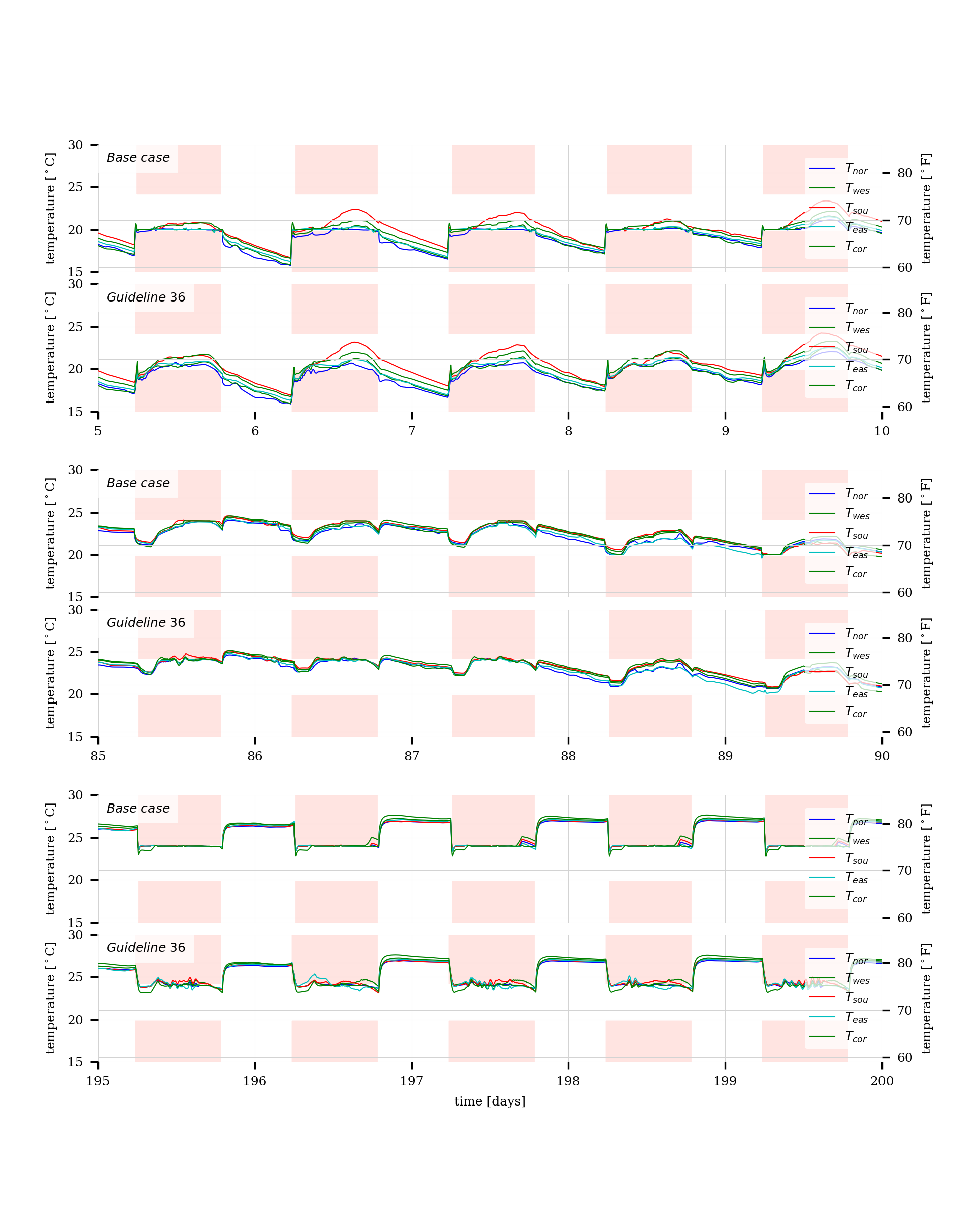
Fig. 13.10 Room air temperatures. The white area indicates the region between the heating and cooling setpoint temperatures.

Fig. 13.10 compares the time trajectories of the room air temperatures. The figures show that the room air temperatures are controlled within the setpoints for both cases. Small set point violations have been observed due to the dynamic nature of the control sequence and the controlled process.

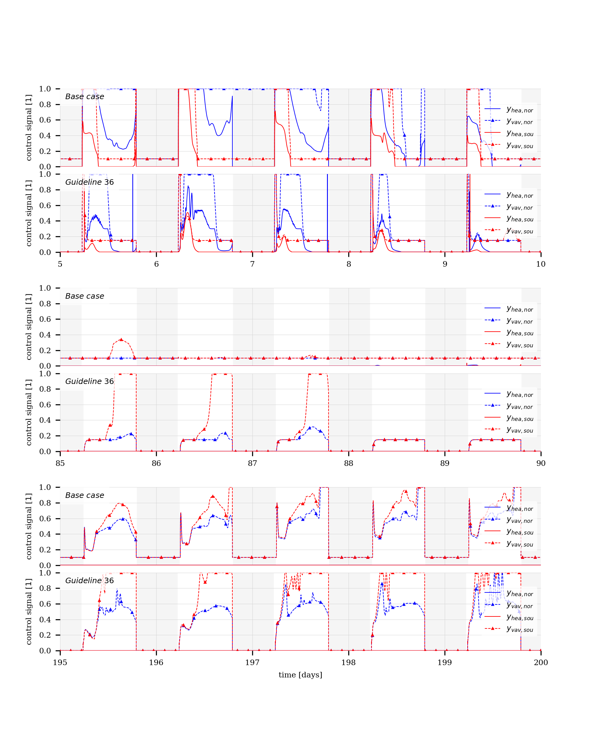
Fig. 13.11 VAV control signals for the north and south zones. The white areas indicate the day-time operation.

Fig. 13.11 shows the control signals of the reheat coils \(y_{hea}\) and the VAV damper \(y_{vav}\) for the north and south zones.

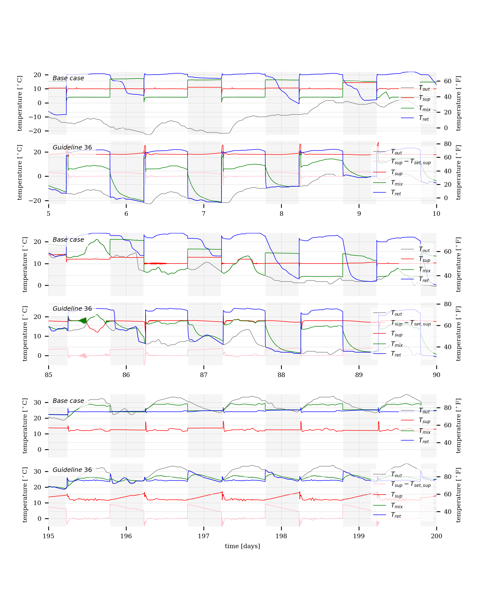
Fig. 13.12 AHU temperatures.

Fig. 13.12 shows the temperatures of the air handler unit. The figure shows the supply air temperature after the fan \(T_{sup}\), its control error relative to its set point \(T_{set,sup}\), the mixed air temperature after the economizer \(T_{mix}\) and the return air temperature from the building \(T_{ret}\). A notable difference is that the Guideline 36 sequence resets the supply air temperature, whereas the base case is controlled for a supply air temperature of \(10^\circ \mathrm C\) for heating and \(12^\circ \mathrm C\) for cooling.

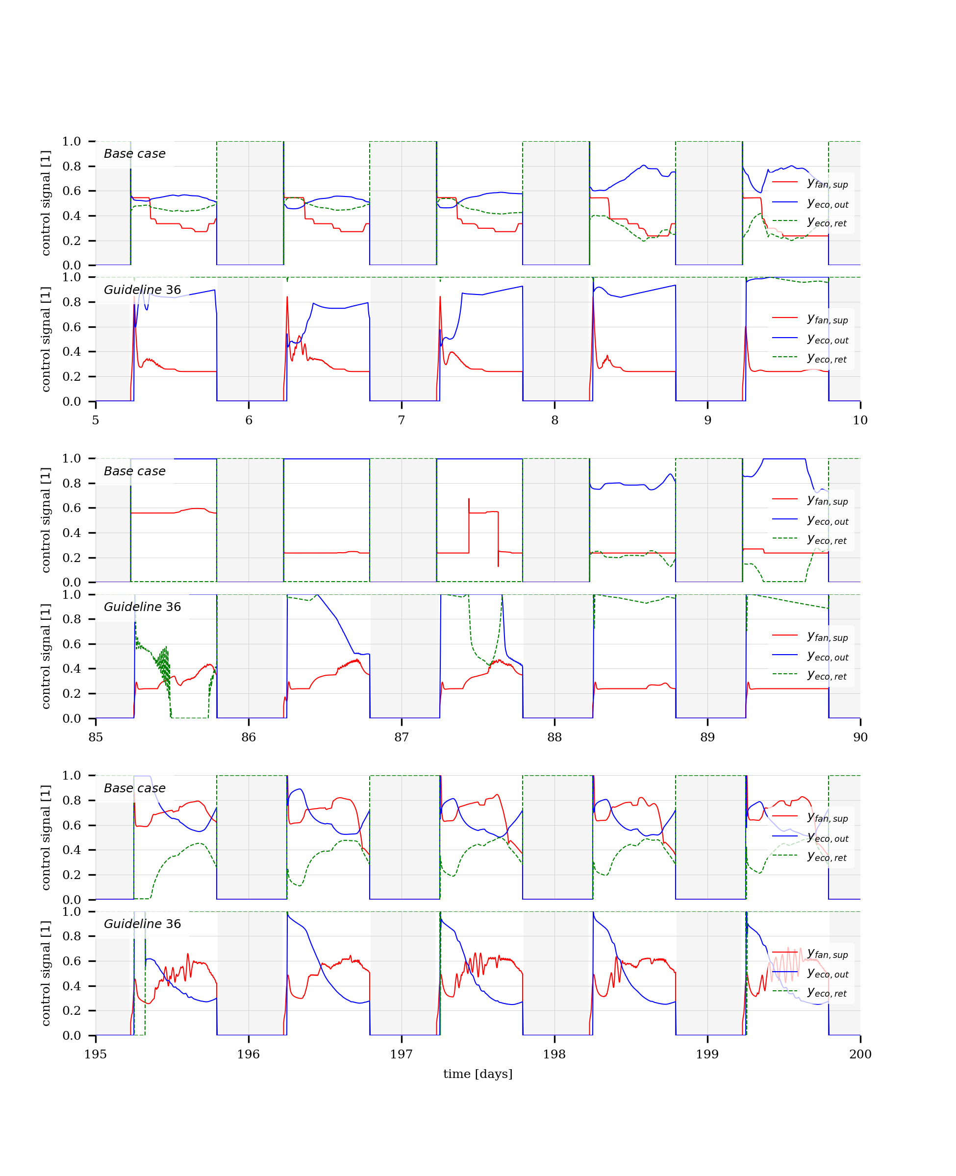
Fig. 13.13 Control signals for the supply fan, outside air damper and return air damper.

Fig. 13.13 show reasonable fan speeds and economizer operation. Note that during the winter days 5, 6 and 7, the outdoor air damper opens. However, this is only to track the setpoint for the minimum outside air flow rate as the fan speed is at its minimum.

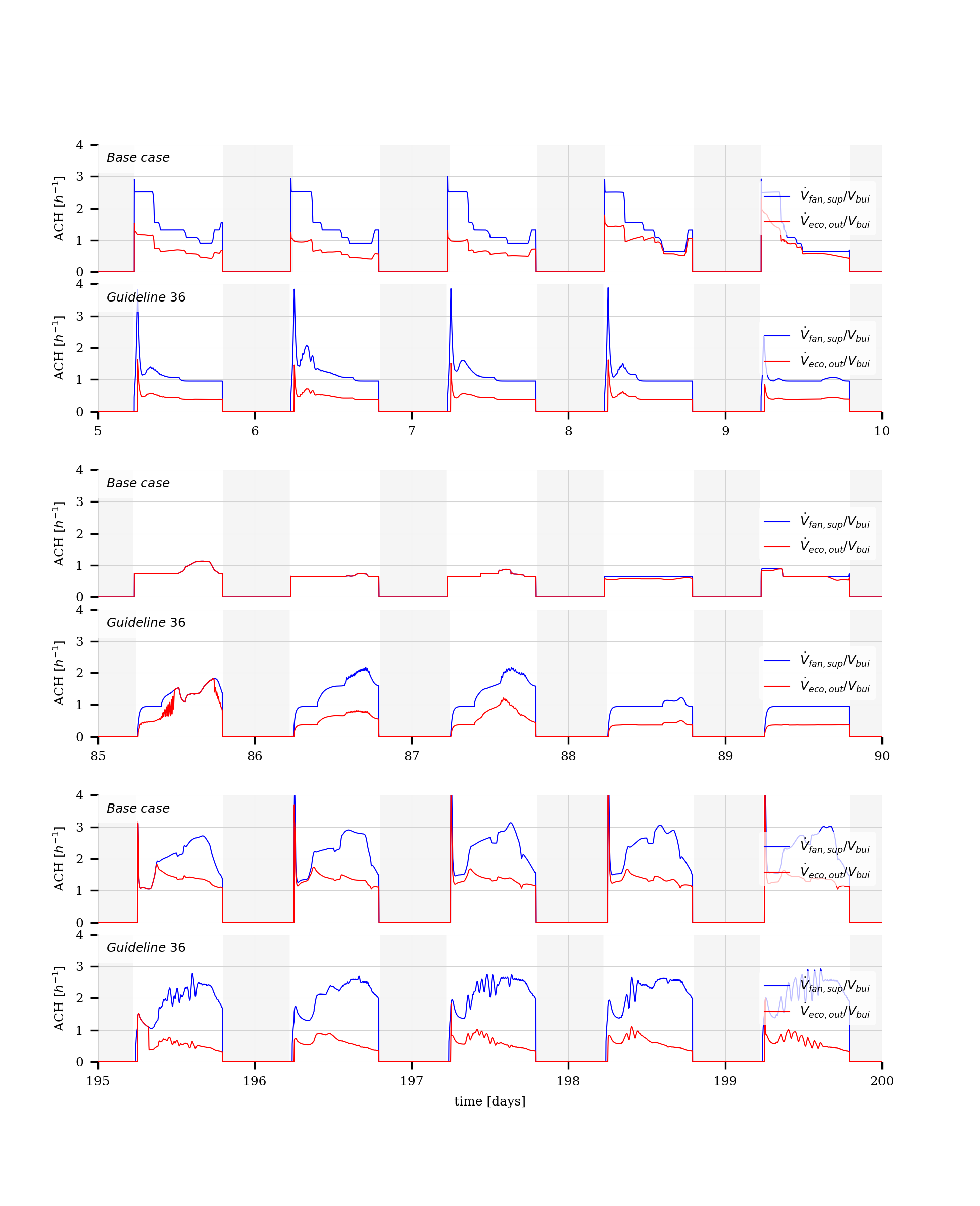
Fig. 13.14 Fan and outside air volume flow rates, normalized by the room air volume.

Fig. 13.14 shows the volume flow rate of the fan \(\dot V_{fan,sup}/V_{bui}\), where \(V_{bui}\) is the volume of the building, and of the outside air intake of the economizer \(\dot V_{eco,out}/V_{bui}\), expressed in air changes per hour. Note that Guideline 36 has smaller outside air flow rates in cold winter and hot summer days. The system has relatively low air changes per hour. As fan energy is low for this building, it may be more efficient to increase flow rates and use higher cooling and lower heating temperatures, in particular if heating and cooling is provided by a heat pump and chiller. We have however not further analyzed this trade-off.

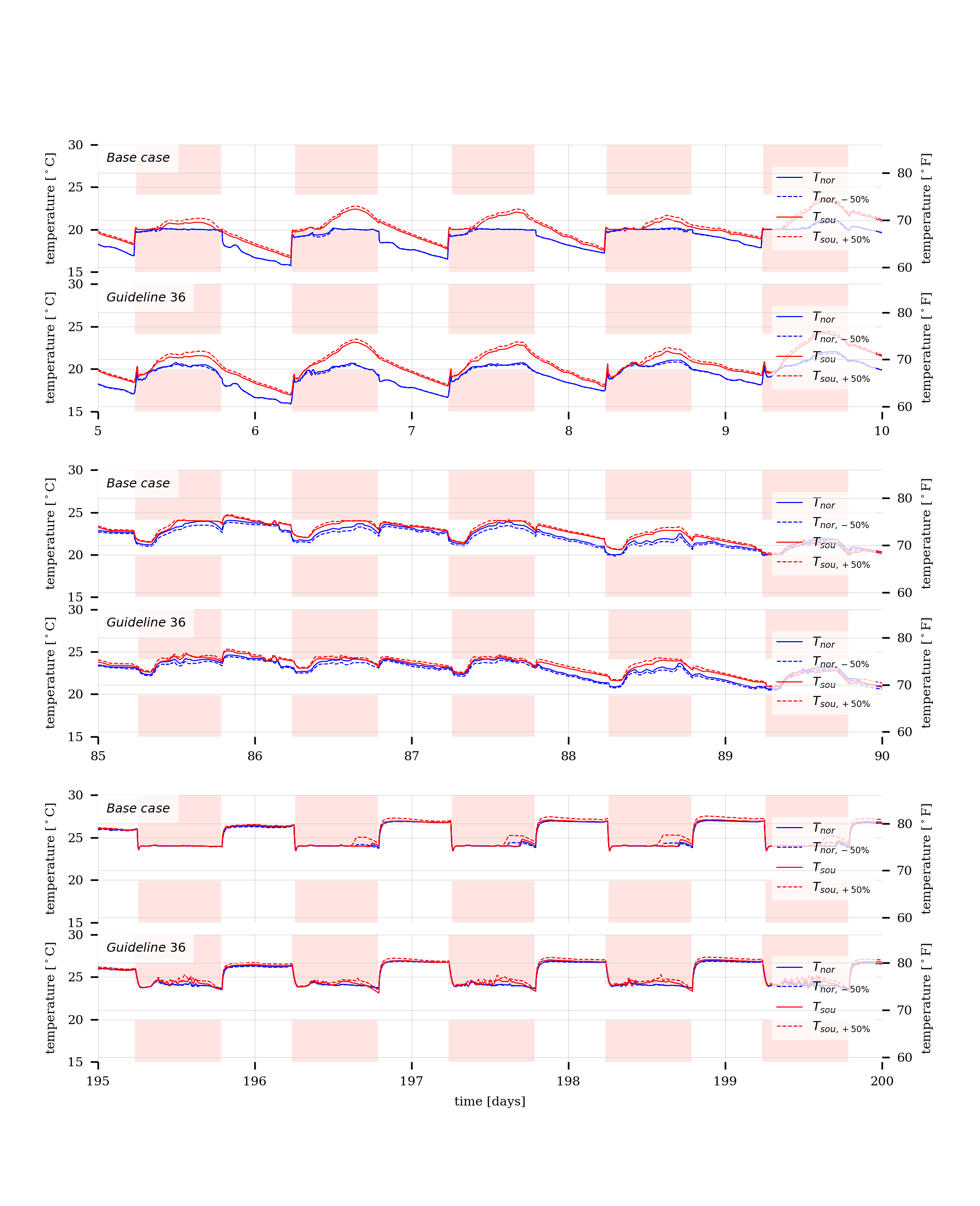
Fig. 13.15 Outdoor air and room air temperatures for the north and south zone with equal internal loads, and with diversity added to the internal loads. The white area indicates the region between the heating and cooling setpoint temperatures.

Fig. 13.15 compares the room air temperatures for the north and south zone for the standard internal loads, and the case where we reduced the internal loads in the north zone by \(50\%\) and increased it by the same amount in the south zone. The trajectories with subscript \(\pm 50\%\) are the simulations with the internal heat gains reduced or increased by \(50\%\). The room air temperature trajectories are practically on top of each other for winter and spring, but the Guideline 36 sequence shows somewhat better setpoint tracking during summer. Both control sequences are comparable in terms of compensating for this diversity, and as we saw in Fig. 13.8, their energy consumption is not noticeably affected.

13.4. Improvement to Guideline 36 Specification

This section describes improvements that we recommend for the Guideline 36 specification, based on the first public review draft [ASHRAE16].

13.4.1. Freeze Protection for Mixed Air Temperature

The sequences have no freeze protection for the mixed air temperature.

Guideline 36 states (emphasis added):

If the supply air temperature drops below \(4.4^\circ \mathrm C\) (\(40^\circ \mathrm F\)) for \(5\) minutes, send two (or more, as required to ensure that heating plant is active) Boiler Plant Requests, override the outdoor air damper to the minimum position, and modulate the heating coil to maintain a supply air temperature of at least \(5.6^\circ\) C (\(42^\circ \mathrm F\)). Disable this function when supply air temperature rises above \(7.2^\circ \mathrm C\) (\(45^\circ \mathrm F\)) for 5 minutes.

Depending on the outdoor air requirements, the mixed air temperature \(T_{mix}\) may be below freezing, which could freeze the heating coil if it has low water flow rate. Note that the Guideline 36 sequence controls based on the supply air temperature and not the mixed air temperature. Hence, this control would not have been active.

Fig. 13.16 shows the mixed air temperature and the economizer control signal for cold climate. The trajectories whose subscripts end in no are without freeze protection control based on the mixed air temperature, as is the case for Guideline 36, whereas for the trajectories that end in with, we added freeze protection that adjusts the economizer to limit the mixed air temperature. For these simulations, we reduced the outdoor air temperature by \(10\) Kelvin (\(18\) Fahrenheit) below the values obtained from the TMY3 weather data. This caused in day 6 and 7 in Fig. 13.16 sub-freezing mixed air temperatures during day-time, as the outdoor air damper was open to provide sufficient fresh air. We also observed that outside air is infiltrated through the AHU when the fan is switched off. This is because the wind pressure on the building causes the building to be slightly below the ambient pressure, thereby infiltrating air through the economizers closed air dampers (that have some leakage). This causes a mixed air temperatures below freezing at night when the fan is off. Note that these temperatures are qualitative rather than quantitative results as the model is quite simplified at these small flow rates, which are about \(0.01\%\) of the air flow rate that the model has when the fan is operating.

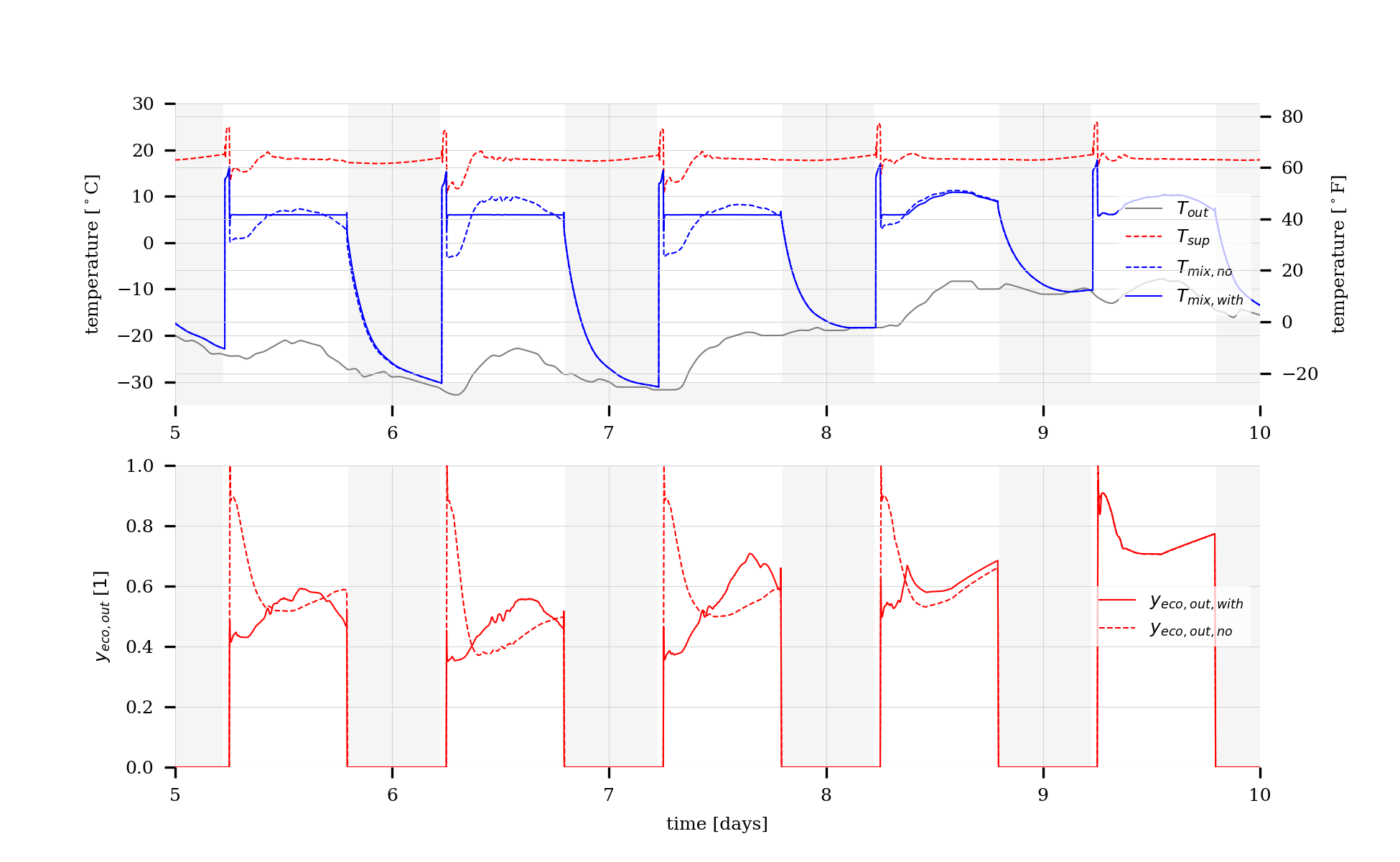
Fig. 13.16 Mixed air temperature and economizer control signal for Guideline 36 case with and without freeze protection.

We therefore recommend adding the following wordings to Guideline 36, which is translated from [Bun86]:

Use a capillary sensor installed after the heating coil. If the temperature after the heating coil is below \(4^\circ C\),

1. enable frost protection by opening the heating coil valve,

2. send frost alarm,

3. switch on pump of the heating coil.

The frost alarm requires manual confirmation.

If the temperature at the capillary sensor exceeds \(6^\circ C\), close the valve but keep the pump running until the frost alarm is manually reset. (Closing the valve avoids overheating).

Recknagel [RSS05] adds further:

1. Add bypass at valve to ensure \(5\%\) water flow.

2. In winter, keep bypass always open, possibly with thermostatically actuated valve.

3. If the HVAC system is off, keep the heating coil valve open to allow water flow if there is a risk of frost in the AHU room.

4. If the heating coil is closed, open the outdoor air damper with a time delay when fan switches on to allow heating coil valve to open.

5. For pre-heat coil, install a circulation pump to ensure full water flow rate through the coil.

13.4.2. Deadbands for Hard Switches

There are various sequences in which the set point changes as a step function of the control signal, such as shown in Fig. 13.5. In our simulations of the VAV terminal boxes, the switch in air flow rate caused chattering. We circumvented the problem by checking if the heating control signal remains bigger than \(0.05\) for \(5\) minutes. If it falls below \(0.01\), the timer was switched off. This avoids chattering. We therefore recommend to be more explicit for where to add hysteresis or time delays.

13.4.3. Averaging Air Flow Measurements

The Guideline 36 sequence does not seem to prescribe that outdoor airflow rate measurements need to be time averaged. As such measurements can fluctuate due to turbulence, we recommend to consider averaging this measurement. In the simulations, we averaged the outdoor airflow measurement over a \(5\) second moving window (in the simulation, this was done to avoid an algebraic system of equations, but, in practice, this would filter measurement noise).

13.4.4. Cross-Referencing and Modularization

For citing individual sections or blocks of the Guideline, it would be helpful if the Guideline where available at a permanent web site as html, with a unique url and anchor to each section. This would allow cross-referencing the Guideline from a particular implementation in a way that allows the user to quickly see the original specification.

As part of such a restructuring, it would be helpful to the reader to clearly state what are the input signals, what are configurable parameters, such as the control gain, and what are the output signals. This in turn would structure the Guideline into distinct modules, for which one could also provide a reference implementation in software.

13.4.5. Lessons Learned Regarding the Simulations

A few lessons regarding simulating such systems have been learned and are reported here. Note that related best practices are also available at https://simulationresearch.lbl.gov/modelica/userGuide/bestPractice.html

• Fan with prescribed mass flow rate: In earlier implementations, we converted the control signal for the fan to a mass flow rate, and used a fan model whose mass flow rate is equal to its control input, regardless of the pressure head. During start of the system, this caused a unrealistic large fan head of \(4000\) Pa (\(16\) inch of water) because the fan increased its mass flow rate faster than the VAV dampers opened. The large pressure drop also lead to large power consumption and hence unrealistic temperature increase across the fan.

• Fan with prescribed pressure head: We also tried to use a fan with prescribed pressure head. Similarly as above, the fan maintains the pressure head as obtained from its control signal, regardless of the volume flow rate. This caused unrealistic large flow rates in the return duct which has very small pressure drops. (Subsequently, we removed the return fan as it is not needed for this system.)

• Time sampling certain physical calculations: Dymola 2018FD01 uses the same time step for all continuous-time equations. Depending on the dynamics, this can be smaller than a second. Since some of the control samples every \(2\) minutes, it has shown to be favorable to also time sample the computationally expensive simulation of the long-wave radiation network in the rooms. Because surface temperatures change slowly, computing it every \(2\) minutes suffices. We expect further speed up can be achieved by time sampling other slow physical processes.

• Non-convergence: In earlier simulations, sometimes the solver failed to converge. This was due to errors in the control implementation that caused event iterations for discrete equations that seemed to have no solution. In another case, division by zero in the control implementation caused a problem. The solver found a way to work around this division by zero (using heuristics) but then failed to converge. Since we corrected these issues, the simulations are stable.

• Too fast dynamics of coil: The cooling coil is implemented using a finite volume model. Heat diffusion among the control volumes of the water and among the control volumes of air used to be neglected as the dominant mode of heat transfer is forced convection if the fan and pump are operating. However, during night when the system is off, the small infiltration due to wind pressure caused in earlier simulations the water in the coil to freeze. Adding diffusion circumvented this problem, and the coil model in the library includes now by default a small diffusive term.

13.5. Discussion and Conclusions

In this case study, the Guideline 36 sequence reduced annual site HVAC energy use by \(30\%\) compared to the baseline implementation with comparable thermal comfort. Such savings are significant, and have been achieved by changes in controls programming only which can relatively easy be deployed in buildings.

Implementing the Guideline 36 sequence was, however, rather challenging due to its complexity caused by the various mode changes, interlocks, timers and cascading control loops. These mode changes, interlocks and dynamic dependencies made verification of the correctness through inspection of the control signals difficult. As a consequence, various programming errors and misinterpretations or ambiguities of the Guideline were only discovered in closed loop simulations, despite of having implemented open-loop test cases for each block of the sequence. We therefore believe it is important to provide robust, validated implementations of the sequences published in Guideline 36. Such implementations would encapsulate the complexity and provide assurances that energy modeler and control providers have correct implementations. With the implementation in the Modelica package Buildings.Controls.OBC.ASHRAE.G36, we made such an implementation and laid out the structure and conventions.

A key short-coming from an implementer point of view was that the sequence was only available in English language, and as an implementation in ALC EIKON of sequences that are “close to the currently used version of the Guideline”. Neither allowed a validation of the CDL implementation because the English language version leaves room for interpretation (and cannot be executed) and because EIKON has quite limited simulation support that is cumbersome to use for testing the dynamic response of control sequences for different input trajectories. Therefore, a benefit of the Modelica implementation is that such reference trajectories can now easily be generated to validate alternate implementations.

A benefit of the simulation based assessment was that it allowed detecting potential issues such as a mixed air temperature below the freezing point (Section 13.4.1) and chattering due to hard switches (Section 13.4.2). Having a simulation model of the controlled process also allowed verification of work-arounds for these issues.

One can, correctly, argue that the magnitude of the energy savings are higher the worse the baseline control is. However, the baseline control was carefully implemented, following our interpretation of ASHRAE’s Sequences of Operation for Common HVAC Systems [ASH06]. While higher efficiency of the baseline may be achieved through supply air temperature reset or different economizer control, such potential improvements were only recognized after seeing the results of the Guideline 36 sequence. Thus, regardless of whether a building is using Guideline 36, having a baseline control against which alternative implementations can be compared and benchmarked is an immensely valuable feature enabled by a library of standardized control sequences. Without a benchmark, one can easily claim to have a good control, while not recognizing what potential savings one may miss.