12. Verification
12.1. Introduction
This section describes how to formally verify whether the control sequence is implemented according to specification. This process would be done as part of the commissioning, as indicated in step 9 in the process diagram Fig. 3.1. For the requirements, see Section 5.3.
For clarity, we note that verification tests whether the implementation of the control sequence conforms with its specification. In contrast, validation would test whether the control sequence, together with the building system, is such that it meets the building owner’s need. Hence, validation would be done in step 2 in Fig. 3.1.
As this step only verifies that the control logic is implemented correctly, it should be conducted in addition to other functional tests, such as tests that verify that sensor and actuators are connected to the correct inputs and outputs, that sensors are installed properly and that the installed mechanical system meets the specification.
12.2. Terminology
We will use the following terminology, see also Section 7 for more details.
By a real controller, we mean a control device implemented in a building automation system.
By a controller, we mean a Modelica block that conforms to the CDL specification and that contains a control sequence.
By input and output, we mean the input connectors (or ports) and output connector (or ports) of a (real) controller.
By input value or output value, we mean the value that is present at an input or output connector at a given time instant.
By time series, we mean a series of values at successive times. The time stamps of the series need not be equidistant, but they need to be non-decreasing, e.g., we allow for time series with two equal time stamps to indicate when a values switches.
By signal, we mean a function that maps time to a value.
By parameter, we mean a configuration value of a controller that is constant, unless it is changed by an operator or by the user who runs the simulation. Typical parameters are sample times, dead bands or proportional gains.
12.3. Scope of the Verification
For OpenBuildingControl, we currently only verify the implementation of the control sequence. The verification is done by comparing output time series between a real controller and a simulated controller for the same input time series and the same control parameters. The comparison checks whether the difference between these time series are within a user-specified tolerance. Therefore, with our tests, we aim to verify that the control provider implemented the sequence as specified, and that it executes correctly.
Outside the scope of our verification are tests that verify whether the I/O points are connected properly, whether the mechanical equipment is installed and functions correctly, and whether the building envelope is meeting its specification.
12.4. Methodology
A typical usage would be as follows: A commissioning agent exports trended control input and output time series and stores them in a CSV file. The commissioning agent then executes the CDL specification for the trended input time series, and compares the following:
Whether the trended output time series and the output time series computed by the CDL specification are close to each other.
Whether the trended input and output time series lead to the right sequence diagrams, for example, whether an airhandler’s economizer outdoor air damper is fully open when the system is in free cooling mode.
Technically, step 2 is not needed if step 1 succeeds. However, feedback from mechanical designers indicate the desire to confirm during commissioning that the sequence diagrams are indeed correct (and hence the original control specification is correct for the given system).
Fig. 12.1 shows the flow diagram for the verification. Rather than using real-time data through BACnet or other protocols, set points, input time series and output time series of the actual controller are stored in an archive, here a CSV file. This allows to reproduce the verification tests, and it does not require the verification tool to have access to the actual building control system. During the verification, the archived time series are read into a Modelica model that conducts the verification. The verification will use three blocks. The block labeled input file reader reads the archived time series, which may typically be in CSV format. As this data may be directly written by a building automation system, its units will differ from the units used in CDL. Therefore, the block called unit conversion converts the data to the units used in the CDL control specification. Next, the block labeled control specification is the control sequence specification in CDL format. This is the specification that was exported during design and sent to the control provider. Given the set points and measurement time series, it outputs the control time series according to the specification. The block labeled time series verification compares these time series with trended control time series, and indicates where the time series differ by more than a prescribed tolerance in time and in control variable value. The block labeled sequence chart creates x-y or scatter plots. These can be used to verify for example that an economizer outdoor air damper has the expected position as a function of the outside air temperature.
Below, we will further describe the blocks in the box labeled verification.

Fig. 12.1 Overview of the verification that tests whether the installed control sequence meets the specification.
Note
We also considered testing criteria such as “whether room temperatures are satisfactory” or “a damper control signal is not oscillating”. However, discussions with design engineers and commissioning providers showed that there is currently no accepted method for turning such questions into hard requirements. We implemented software that tests criteria such as “Room air temperature shall be within the setpoint \(\pm 0.5\) Kelvin for at least 45 min within each \(60\) minute window.” and “Damper signal shall not oscillate more than \(4\) times per hour between a change of \(\pm 0.025\) (for a \(2\) minute sample period)”. Software implementations of such tests are available on the Modelica Buildings Library github repository, commit 454cc75.
Besides these tests, we also considered automatic fault detection and diagnostics methods that were proposed for inclusion in ASHRAE RP-1455 and Guideline 36, and we considered using methods such as in [Ver13] that automatically detect faulty regulation, including excessively oscillatory behavior. However, as it is not yet clear how sensitive these methods are to site-specific tuning, and because field tests are ongoing in a NIST project, we did not implement them.
12.5. Modules of the Verification Test
To conduct the verification, the following models and tools are used.
12.5.1. CSV File Reader
To read CSV files, the data reader Modelica.Blocks.Sources.CombiTimeTable
from the Modelica Standard Library
can be used. It requires the CSV file to have the following structure:
#1
# comment line
double tab1(6,2)
# time in seconds, column 1
  0   0
  1   0
  1   1
  2   4
  3   9
  4  16
Note, that the first two characters in the file need to be #1
(a line comment defining the version number of the file format).
Afterwards, the corresponding matrix has to be declared with type
double, name and dimensions.
Finally, in successive rows of the file, the elements
of the matrix have to be given.
The elements have to be provided as a sequence of numbers
in row-wise order (therefore a matrix row can span several
lines in the file and need not start at the beginning of a line).
Numbers have to be given according to C syntax
(such as 2.3, -2, +2.e4). Number separators are spaces,
tab, comma, or semicolon.
Line comments start with the hash symbol (#) and can appear everywhere.
12.5.2. Unit Conversion
Building automation systems store physical quantities in various units.
To convert them to the units used by Modelica and hence also by CDL,
we developed the package Buildings.Controls.OBC.UnitConversions.
This package provides blocks that convert between SI units
and units that are commonly used in the HVAC industry.
12.5.3. Comparison of Time Series Data
We have been developing a tool called funnel to conduct time series comparison. The tool imports two CSV files, one containing the reference data set and the other the test data set. Both CSV files contain time series that need to be compared against each other. The comparison is conducted by computing a funnel around the reference curve. For this funnel, users can specify the tolerances with respect to time and with respect to the trended quantity. The tool then checks whether the time series of the test data set is within the funnel and computes the corresponding exceeding error curve.
The tool is available from https://github.com/lbl-srg/funnel.
It is primarily intended to be used by means of a Python binding. This can be done in two ways:
Import the module
pyfunneland use thecompareAndReportandplot_funnelfunctions. Fig. 12.2 shows a typical plot generated by use of these functions.Run directly the Python script from terminal. For usage information, run
python pyfunnel.py --help.
For the full documentation of the funnel software, visit https://github.com/lbl-srg/funnel

Fig. 12.2 Typical plot generated by pyfunnel.plot_funnel for comparing test and reference time series.
12.5.4. Verification of Sequence Diagrams
To verify sequence diagrams we developed the Modelica package
Buildings.Utilities.IO.Plotters.
Fig. 12.3 shows an example in which this block is used to produce the sequence
diagram shown in Fig. 12.4. While in this example, we used the control
output time series of the CDL implementation, during commissioning,
one would use the controller output time series from the building automation system.
The model is available from the Modelica Buildings Library, see the model
Buildings.Utilities.Plotters.Examples.SingleZoneVAVSupply_u.

Fig. 12.3 Modelica model that verifies the sequence diagram.
On the left are the blocks that generate the control input time series.
In a real verification, these would be replaced with a file reader that
reads data that have been archived by the building automation system.
In the center is the control sequence implementation.
Some of its output values are converted to degree Celsius, and then fed to the
plotters on the right that generate a scatter plot for the temperatures
and a scatter plot for the fan control signal.
The block labeled plotConfiguration configures
the file name for the plots and the sampling interval.

Fig. 12.4 Control sequence diagram for the VAV single zone control sequence from ASHRAE Guideline 36.
Simulating the model shown in Fig. 12.3 generates an html file that contains the scatter plots shown in Fig. 12.5.
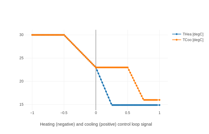
Fig. 12.5 Scatter plots that show the control sequence diagram generated from the simulated sequence.
12.6. Example
In this example we validated a trended output time series of a control sequence that defines the cooling coil valve position. The cooling coil valve sequence is a part of the ALC EIKON control logic implemented in building 33 on the main LBNL campus in Berkeley, CA. The subsequence is shown in Fig. 12.6. It comprises a PI controller that tracks the supply air temperature, an upstream subsequence that enables the controller and a downstream output limiter that is active in case of low supply air temperatures.
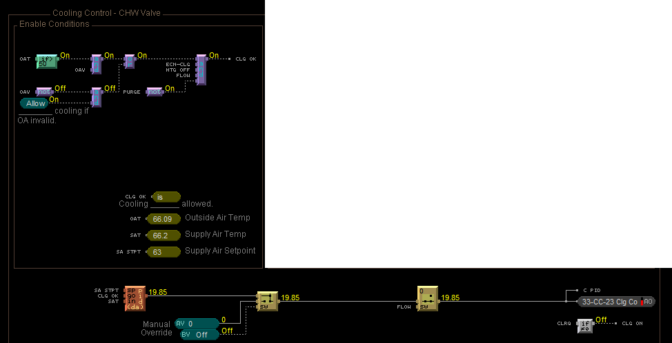
Fig. 12.6 ALC EIKON specification of the cooling coil valve position control sequence.

Fig. 12.7 CDL specification of the cooling coil valve position control sequence.
We created a CDL specification of the same cooling coil valve position control sequence, see Fig. 12.7, to validate the trended output time series. We trended controller inputs and outputs in 5 second intervals for
Supply air temperature in [F]
Supply air temperature setpoint in [F]
Outdoor air temperature in [F]
VFD fan enable status in [0/1]
VFD fan feedback in [%]
Cooling coil valve position, which is the output of the controller, in [%].
The trended input and output time series were processed with a script that converts them to the format required by the data readers. The data used in the example begins at midnight on June 7 2018. In addition to the trended input and output time series, we recorded all parameters, such as the hysteresis offset (see Fig. 12.8) and the controller gains (see Fig. 12.9), to use them in the CDL controller.
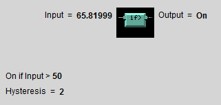
Fig. 12.8 ALC EIKON outdoor air temperature hysteresis to enable/disable the controller.
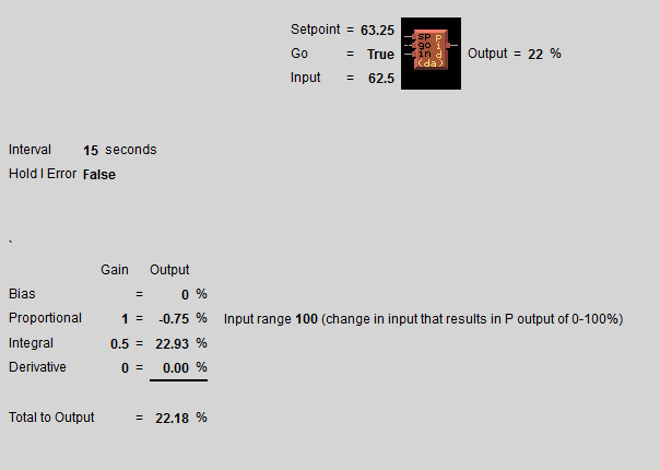
Fig. 12.9 ALC EIKON PI controller parameters.
We configured the CDL PID controller parameters such that they correspond to the parameters of the ALC PI controller. The ALC PID controller implementation is described in the ALC EIKON software help section, while the CDL PID controller is described in the info section of the model Buildings.Controls.OBC.CDL.Reals.PID. The ALC controller tracks the temperature in degree Fahrenheit, while CDL uses SI units. An additional implementation difference is that for cooling applications, the ALC controller uses direct control action, whereas the CDL controller needs to be configured to use reverse control action, which can be done by setting its parameter reverseAction=true. Furthermore, the ALC controller outputs the control action in percentages, while the CDL controller outputs a signal between \(0\) and \(1\). To reconcile the differences, the ALC controller gains were converted for CDL as follows: The proportional gain \(k_{p,cdl}\) was set to \(k_{p,cdl} = u \, k_{p,alc}\), where \(u=9/5\) is a ratio of one degree Celsius (or Kelvin) to one degree Fahrenheit of temperature difference. The integrator time constant was converted as \(T_{i,cdl} = k_{p,cdl} \, I_{alc}/(u \, k_{i,alc})\). Both controllers were enabled throughout the whole validation time.
Fig. 12.10 shows the
Modelica model that was used to conduct the verification. On the left hand side
are the data readers that read the trended input and output time series
from files. Next are unit converters, and a conversion for the fan status
between a real value and a boolean value. These data are fed into the instance labeled
cooValSta, which contains the control sequence
as shown in Fig. 12.7. The plotters on the right hand side then
compare the simulated cooling coil valve position with the trended time series.

Fig. 12.10 Modelica model that conducts the verification.
Fig. 12.11,
which was produced by the Modelica model using blocks from the
Buildings.Utilities.Plotters package,
shows the trended input temperatures for the
control sequence, the trended and simulated cooling valve control signal
for the same time period, which are practically on top of each other,
and a correlation error between the
trended and simulated cooling valve control signal.
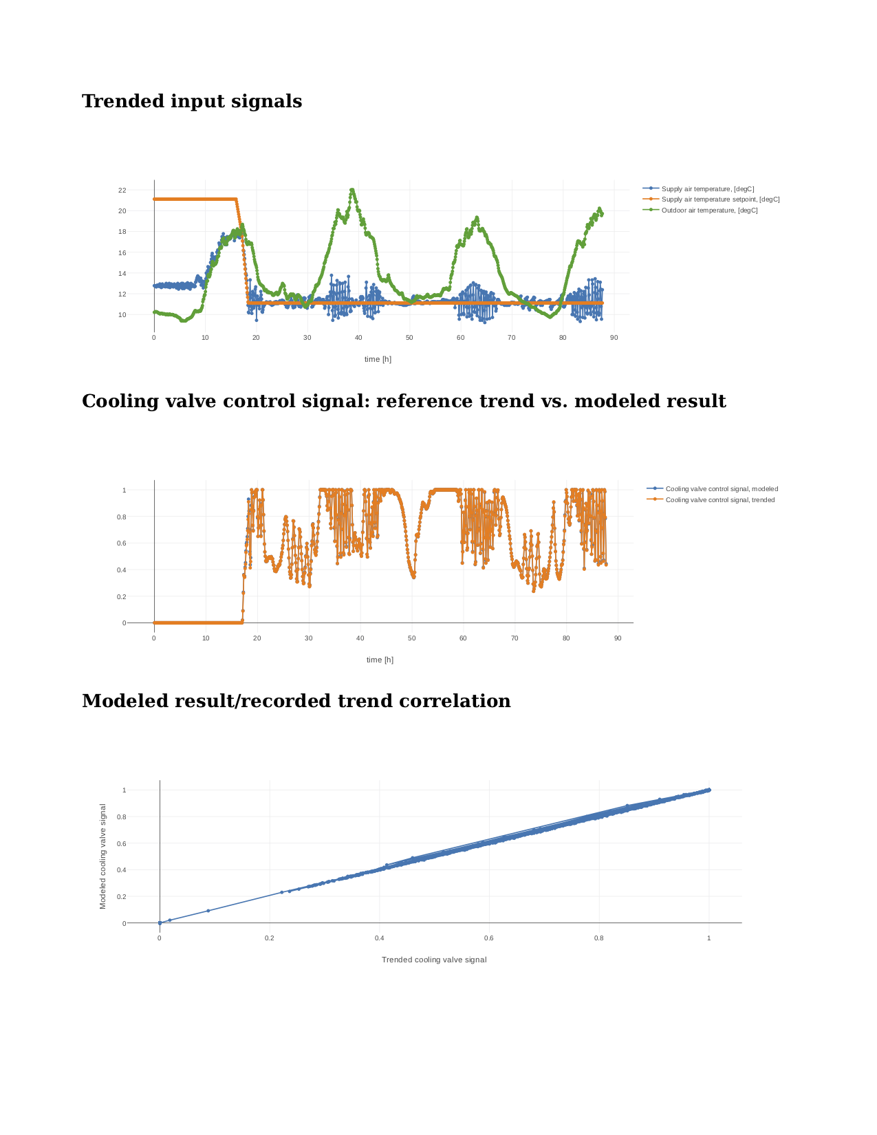
Fig. 12.11 Verification of the cooling valve control signal between ALC EIKON computed signal and simulated signal.
The difference in modeled vs. trended results is due to the following factors:
ALC EIKON uses a discrete time step for the time integration with a user-defined time step length, whereas CDL uses a continuous time integrator that adjusts the time step based on the integration error.
ALC EIKON uses a proprietary algorithm for the anti-windup, which differs from the one used in the CDL implementation.

Fig. 12.12 Verification of the cooling valve control signal with the funnel software (error computed with an absolute tolerance in time of 1 s and a relative tolerance in y of 1%).
Despite these differences, the computed and the simulated control signals show good agreement, which is also demonstrated by verifying the time series with the funnel software, whose output is shown in Fig. 12.12.
12.7. Specification for Automating the Verification
The example Section 12.6 describes a manual process of composing the verification model and executing the verification process. In this section, we provide specifications for how this process can be automated. The automated workflow uses the same modules as in Section 12.6, except that the unit conversion will need to be done by the tool that reads the CSV files and sends data to the Building Automation System, and that reads data from the Building Automation System and writes them to the CSV files. This design decision has been done because CDL provides all required unit information, but this is not the case in general for a building automation system. Moreover, in the process described in this section, the CSV files will be read directly by the Modelica simulation environment rather than using the CSV file reader described in Section 12.5.1.
12.7.1. Use Cases
We address two use cases. Both uses cases verify conformance of the time series generated by a control control sequence specified in CDL against the time series of an implementation of a real controller. For both use cases, the precondition is that one control sequence, or several control sequences, are available in CDL. The output will be a report that describes whether the real implementation conforms to the CDL implementation within a user-specified error tolerance. The difference between the two uses cases is as follows: In scenario 1, the CDL model contains the controller that is connected to upstream blocks that generate the control input time series. The time series from this CDL model will be used to test the real controller. In scenario 2, data trended from a real controller will be used to verify the controller against the output time series of its CDL specification, using as inputs and parameters of the CDL specification the trended time series and parameters of the real controller.
To conduct the verification, the following three steps will be conducted:
Specify the test setup,
generate data from the real controller, and
produce the test results.
Next, we will describe the specifications for the two scenarios. The specifications focus on the CDL side. In addition, for Scenario 1, steps 5 & 6, and for Scenario 2, steps 3 & 4, a data collection tool need to be developed that utilizes the JSON and CSV files described below and does the following to generate the data from the real controller:
Identifies which objects in the building automation system match with the desired collection.
Shows the user a list of all objects that don’t match and a list of objects from the building automation system and allows for the user to manually match them.
Sets up the data collection.
Starts collecting data at the desired intervals.
Store the data.
Export the desired data in the format specified below.
Note
In support of this step, work is ongoing in exporting semantic information from the CDL implementation.
12.7.2. Scenario 1: Control Input Obtained by Simulating a CDL Model
For this scenario, we verify whether a real controller outputs time series that are similar to the time series of a controller that is implemented in a CDL model. The inputs of the real controller will be connected to the time series that were exported when simulating a controller that is connected to upstream blocks that generate the control input time series.
An application of this use case is to test whether a controller complies with the sequences specified in CDL for a given input time series and control parameters, either as part of verifying correct implementation during control development, or verifying correct implementation in a Building Automation System that allows overwriting control input time series.
We have also developed a verification tool for verifying the control sequences implemented in a controller using CDL.
For this scenario, we are given the following data:
A list of CDL models to be tested.
Relative and absolute tolerances, either for all output variables, or optionally for individual output variables of the sequence.
Optionally, a boolean variable in the model that we call an indicator variable. An indicator variable allows to indicate when to pause a test, such as during a fast transient, and when to resume the test, for example when the controls is expected to have reached steady-state. If its value is
true, then the output should be tested at that time instant, and if it isfalse, the output must not be tested at that time instant.
For example, consider the validation test
OBC.ASHRAE.G36.AHUs.SingleZone.VAV.SetPoints.Validation.Supply_u.
and suppose we want to verify the sequences of its instances setPoiVAV and setPoiVAV1.
To do so, we first write a specification
as shown in Listing 12.1.
{
  "references": [
    {
      "model": "Buildings.Controls.OBC.ASHRAE.G36.AHUs.SingleZone.VAV.SetPoints.Validation.Supply_u",
      "generateJson": false,
      "sequence": "setPoiVAV",
      "pointNameMapping": "realControllerPointMapping.json",
      "runController": false,
      "controllerOutput": "test/real_outputs.csv"
    },
    {
      "model": "Buildings.Controls.OBC.ASHRAE.G36.AHUs.SingleZone.VAV.SetPoints.Validation.Supply_u",
      "generateJson": true,
      "sequence": "setPoiVAV1",
      "pointNameMapping": "realControllerPointMapping.json",
      "runController": true,
      "controllerOutput": "test/real_outputs.csv",
      "outputs": {
        "setPoiVAV1.TSup*": { "atoly": 0.5 }
      },
      "indicators": {
        "setPoiVAV1.TSup*": [ "fanSta.y" ]
      },
      "sampling": 60
    }
  ],
  "modelJsonDirectory": "test",
  "tolerances": { "rtolx": 0.002, "rtoly": 0.002, "atolx": 10, "atoly": 0 },
  "sampling": 120,
  "controller": {
    "networkAddress": "192.168.0.115/24",
    "deviceAddress": "192.168.0.227",
    "deviceId": 240001
  }
}
This specifies two tests, one for the controller setPoiVAV and one for setPoiVAV1.
In this example, setPoiVAV and setPoiVAV1 happen to be the same sequence, but their
input time series and/or parameters are different, and therefore their output time series will be different.
The generateJson flag will determine if the json translation for the specified model under test
must be generated during the test using the modelica-json tool.
If it is set to false, the software assumes that the json translation is already present in modelJsonDirectory.
The test for setPoiVAV will use the globally specified tolerances, and use
a sampling rate of \(120\) seconds. The mapping of the variables to the I/O points of the real controller
is provided in the file realControllerPointMapping.json, shown in Listing 12.2.
The test setPoiVAV will not run
the controller during the test because of the specification runController = false.
Rather, it will use the saved results test/real_outputs.csv from a previous run.
The test for setPoiVAV1 will use different tolerances on each output
variable that matches the regular expression setPoiVAV1.TSup*.
Moreover, for each variable that matches the regular
expression setPoiVAV1.TSup*, the verification will be suspended whenever
fanSta.y = false. The sampling rate is \(60\) seconds. This test will also use
realControllerPointMapping.json to map the variables to points of the real controller.
Because runController = true, this test
will run the controller in real-time and save the time-series of the output
variables in the file specified by controllerOutput.
The real controller’s network configuration can be found
under the controller section of the configuration.
The networkAddress is the controller’s
BACnet subnet, the deviceAddress is the controller’s IP address and
the deviceId is the controller’s BACnet
device identifier.
The tolerances rtolx and atolx are relative and absolute tolerances in the independent
variable, e.g., in time, and rtoly and atoly are relative and absolute tolerances
in the control output variable.
[
   {
       "cdl": {   "name": "TZonCooSetOcc",                 "unit": "K",    "type": "float"},
       "device": {"name": "Occupied Cooling Setpoint_1",   "unit": "degF", "type": "float"}
   },
   {
       "cdl": {   "name": "TZonHeaSetOcc",                 "unit": "K",    "type": "float"},
       "device": {"name": "Occupied Heating Setpoint_1",   "unit": "degF", "type": "float"}
   },
   {
       "cdl": {   "name": "TZonCooSetUno",                 "unit": "K",    "type": "float"},
       "device": {"name": "Unoccupied Cooling Setpoint_1", "unit": "degF", "type": "float"}
   },
   {
       "cdl": {   "name": "TZonHeaSetUno",                 "unit": "K",    "type": "float"},
       "device": {"name": "Unoccupied Heating Setpoint_1", "unit": "degF", "type": "float"}
   },
   {
       "cdl": {   "name": "setAdj",                        "unit": "K",    "type": "float"},
       "device": {"name": "setpt_adj_1",                   "unit": "degF", "type": "float"}
   },
   {
       "cdl": {   "name": "heaSetAdj",                     "unit": "K",    "type": "float"},
       "device": {"name": "Heating Adjustment_1",          "unit": "degF", "type": "float"}
   },
   {
       "cdl": {   "name": "uOccSen",                                       "type": "int"},
       "device": {"name": "occ_sensor_bni_1",                              "type": "bool"}
   },
   {
       "cdl": {   "name": "uWinSta",                                       "type": "int"},
       "device": {"name": "window_sw_1",                                   "type": "bool"}
   },
   {
       "cdl": {   "name": "TZonCooSet",                   "unit": "K",    "type": "float"},
       "device": {"name": "Effective Cooling Setpoint_1", "unit": "degF", "type": "float"}
   },
   {
       "cdl": {   "name": "TZonHeaSet",                   "unit": "K",    "type": "float"},
       "device": {"name": "Effective Heating Setpoint_1", "unit": "degF", "type": "float"}
   }
]
Listing 12.2 is an example of the pointNameMapping file.
It is a list of dictionaries, with each dictionaries having two parts:
The cdl part specifies the name, the unit and the
type of the point in the CDL sequence.
Similarly, the device part specifies this information for the corresponding
point in the real controller.
The type refers to the data type of the variable in the specific context, i.e., in CDL or
in the actual controller.
It should also be noted that some points may not have a unit, but only have a type.
For example, the input uOccSen is a CDL point that is 1 if there is occupancy and
0 otherwise.
To create test input and output time series, we generate CSV files. This needs to be done for each
controller (or control sequence) under test, and we will explain it only for the controller setPoiVAV.
For brevity, we call OBC.ASHRAE.G36.AHUs.SingleZone.VAV.SetPoints.Validation.Supply_u
simply Supply_u.
Once we have the configuration and the pointNameMapping file set up, the sequence verification
(handled by the verification tool) goes through the
following steps:
Generate a json translation of the modelica code. Currently the verification tool does invoke the
modelica-jsontool from within itself, depending on thegenerateJsonflag in the configuration (and stores the output in the directory mentioned undermodelJsonDirectory). The user can themselves invoke themodelica-jsontool using:node app.js -f Buildings/Controls/OBC/ASHRAE/G36/AHUs/SingleZone/VAV/SetPoints/Validation/Supply_u.mo -o json -d test
This will produce
Supply_u.json(file name is abbreviated) in the output directorytest. See https://github.com/lbl-srg/modelica-json for the json schema.From
Supply_u.json, extract all input and output variable declarations of the instancesetPoiVAVand generate an I/O list . The tool also extracts public parameters of the instancesetPoiVAVand stores them. For this sequence, the public parameters areTSupSetMax,TSupSetMin,yHeaMax,yMinandyCooMax.Obtain reference time series by simulating
Supply_u.mowith time series of all input, output and indicator time series. The verification tool accomplishes this by using the free open-source tool OpenModelica. The verification tool will create Modelica scripts to translate the model, followed by one to simulate the model. This will produce aSupply_u_res.matfile, from which the tool will extract the timeseries of the inputs and the outputs and store it asSupply_u_res.csv.More information about the python script used to run the OpenModelica simulation can be found at software/verification/openmodelica_sim.py.
Using the input and output variables extracted for the sequence
setPoiVAV, the verification tool then separates the input and the output timeseries (reference outputs).Steps 6 and 7 are applied only if
runControllerflag in the test configuration file is set toTrue. Else, the tool will use the real outputs previously generated by the controller and saved in the file mentioned undercontrollerOutput. Proceed to step 8.If the
runControllerflag isTrue, the verification applies the parameters that have been extracted to the real controller, and runs the real controller for the input time series extracted in the step above. Using thepointNameMappingfile, the tool will also handle the unit conversions and the type conversions on the time series as needed for the controller under test.As the controller is being set different input values, the output variables are trended and saved to
setPoiVAV_real_outputs.csv. The point names, units and the types of the output time series will also be converted to match the CDL input timeseries as specified in thepointNameMappingfile.Produce the test results by running the funnel software (https://github.com/lbl-srg/funnel) for each time series of the output variables generated by the controller (
setPoiVAV_output.csvor file incontrollerOutput) against the corresponding output variables generated by the CDL simulation. Before sending the time series to the funnel software, set the value of the reference and the controller output to zero whenever the indicator function is zero for that time stamp. This will exclude the value from the verification. This will give, for each time series, output files that show where the error exceeds the specified tolerance.
The sequence above can be run for each test case, and the results from step 8 are to be used to generate a test report for all tested sequences.
An example of a sequence under test, along with real inputs from a controller have been included in the verification tool software. Please see software/verification for how to automate this process.
12.7.3. Scenario 2: Control Input Obtained by Trending a Real Controller
For this scenario, we verify whether a real controller produces time series that are similar to the time series of a controller that is implemented in a CDL model. As control input time series, the time series trended from the real controller are used.
An applications of this use case is to test if a controller complies with the sequences specified in CDL for already trended data.
For this scenario, we are given the following data:
The CDL class name of the control sequence to be tested, in our example
Buildings.Controls.OBC.ASHRAE.G36.AHUs.SingleZone.VAV.SetPoints.Supply.Relative and absolute tolerances, either for all output variables, or optionally for individual output variables of the sequence.
Therefore, a test specification looks as shown in Listing 12.3, which is identical to Listing 12.1, except that the elements indicator and sampling are removed because a sequence cannot have an indicator function, and because CDL simulators control the accuracy and hence a sampling time step is not needed. However, a time series for an indicator function can be provided, see step 4 below.
references : [
  { "model": "Buildings.Controls.OBC.ASHRAE.G36.AHUs.SingleZone.VAV.SetPoints.Supply" },
    "tolerances": {"atoly": 0.5, "variable": "TSup*" },
  }
],
"tolerances": {"rtolx": 0.002, "rtoly": 0.002, "atolx": 10, "atoly": 0},
Note that we allow for multiple entries in references to allow testing more than one sequence.
To create test input and output time series, we generate again CSV files. This needs to be done for each control sequence. Here, we only explain it for the one sequence shown in Listing 12.3.
The procedure is as follows:
Produce the json file
Supply.json(name abbreviated) by runningmodelica-jsonasnode app.js -f Buildings/Controls/OBC/ASHRAE/G36/AHUs/SingleZone/VAV/SetPoints/Supply.mo -o json -d test1
Generate the list of input and output variable declarations
reference_io.jsonand the parameter listreference_parameters.jsonas in Step 2 in Section 12.7.2.Trend the input and output time series specified in
reference_io.jsonfrom the real controller, trending as input time series whatever the controller receives from the actual building automation system. (However, make sure there is reasonable excitation of the control input.)Convert the trended input time series of the real controller to the units specified in
reference_io.json, and write the converted input time series to a new filereference_input.csv, using the formattime, uHea, uCoo, TZonSet, TZon, TOut, uFan 0, 1, 0, 293.15, 292.15, 283.15, 1 60, 0.5, 0, 293.15, 292.15, 283.15, 1 120, 0, 0.5, 293.15, 292.15, 283.15, 1 180, 0, 1, 293.15, 292.15, 283.15, 1 3600, 0, 1, 293.15, 292.15, 283.15, 1
where the first column is time in seconds.
Do the same for the trended output time series of the real controller and store them in the new file
controller_output.csvthat has the same format asreference_input.csvOptionally, also store one or several indicator time series in
indicator.csv, with the header of each time series being the name of the control output variable whose verification should be suspended whenever the indicator time series is0at that time instant. For example, to suspend the verification of an output calledTSupCoobetween \(t=120\) and \(t=600\) seconds, the fileindicator.csvlooks liketime, TSupCoo 0, 1 120, 0 600, 1
Convert the parameter values for
TSupSetMax,TSupSetMin,yHeaMax,yMinandyCooMaxas used in the real controller to the units specified inreference_parameters.jsonand store them in a text filereference_parameters.txt. For our example, suppose this file isTSupSetMax=303.15 TSupSetMin=289.15 yHeaMax=0.7 yMin=0.3 yCooMax=1
Simulate the sequence specified in the class definition
Supply.mo, using the parameter values fromreference_parameters.txtand the input time series fromreference_input.csv.This can be accomplished with the free open-source tool OpenModelica by running
#~/bin/bash
set -e
export OPENMODELICALIBRARY=`pwd`:/usr/lib/omlibrary
python3 -i simulateCDL.py
rm -f Buildings.* 2&> /dev/null
with the file
simulateCDL.pybeingimport shutil import os from OMPython import OMCSessionZMQ model="Buildings.Controls.OBC.ASHRAE.G36.AHUs.SingleZone.VAV.SetPoints.Supply" parameters="(TSupSetMax=303.15, TSupSetMin=289.15, yHeaMax=0.7, yMin=0.3, yCooMax=1)" omc = OMCSessionZMQ() omc.sendExpression("loadModel(Buildings)") omc.sendExpression("simulate({}, startTime=0, stopTime=3600, simflags=\"-csvInput reference_input.csv\", outputFormat=\"csv\")".format(model)) shutil.move("{}_res.csv".format(model), "reference.csv")
This will produce the CSV file
reference.csvthat contains all control input and output time series.Produce the test results as in Step 7 in Section 12.7.2.
The sequence above can be run for each test case, and the results from step 7 are to be used to generate a test report for all tested sequences.